ISE Cryptography — Lecture 02

Stream Ciphers

The story so far…

Classical cryptography!
- Don’t use it in the modern world, though.
Cryptanalysis!
- Cracking classical ciphers (and appreciating awful alliteration).
Perfect security!
- Awesome, but about as useful as a chocolate teapot.
Semantic security!
- Less-than-perfect, but practical.
Today’s themes: using short keys, proving security, and variable-length messages
- All of this (and more) as we look at stream ciphers…

Fix the One-Time Pad?

Starting the day with some déjà vu

The One-Time Pad

Everyone remember the one-time pad from last time?
What does it use as…
- The encryption function?
- The decryption function?
- The key?
What constraints apply when using it?
Is it…
- Perfectly secure?
- Semantically secure?
- IND-CPA secure? (a term we’ll define later)
- Secure against message recovery attacks?
Why can’t we just use it for everything and skip the rest of cryptography?

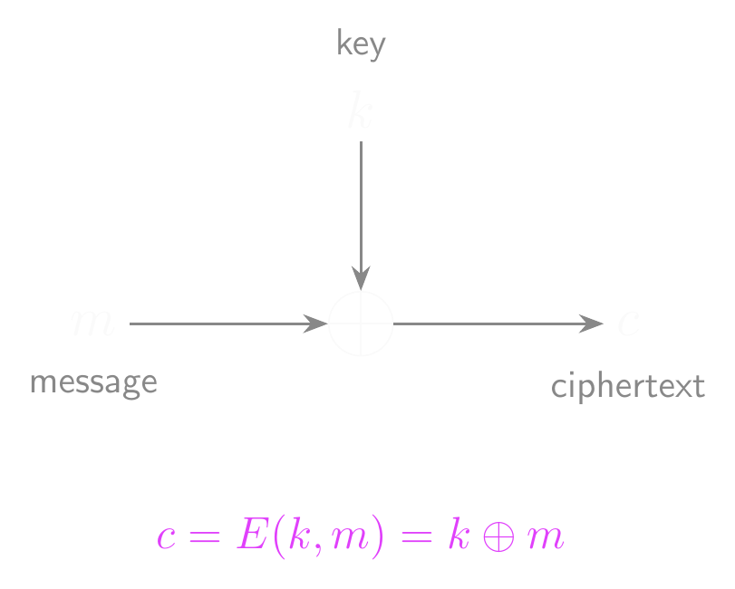
One-Time Pad: Encryption

The Key Problem

Needing a key as long as the message makes the one-time pad almost useless.
- How can we share it securely?
- And it’s only good for a single message!
- The USSR (Venona) and Microsoft (PPTP) both fell victim to that particular issue!
We need a way to use a short, fixed-length key to encrypt/decrypt
- But we can’t do this with the one-time pad!
- Why can’t we just repeat the short key end-to-end for long messages?
If an attacker can predict parts of the key…
- They can break semantic security!
How did you generate keys for last week’s lab/tutorial?
- Probably with Python’s secrets module, right?
- So we can generate them, but we’d still have to share them…

The Integrity Problem

A passive attacker can’t read messages encrypted with a one-time pad…
- But an active attacker can cause a lot of trouble.
- The one-time pad is malleable
You have no way of verifying whether the message you’ve decrypted is the one that was sent! It could have been…
- Modified in transit
- Stored and replayed later
- Cut into chunks and selectively reassembled
Also vulnerable to bit-flipping attacks
- Flipping a bit in the ciphertext flips that same bit in the plaintext
An attacker can make predictable changes to the plaintext…
- Even if they can’t read it!
Extremely dangerous if the format of the message is known

Solutions

We’re going to leave the integrity/malleability problem alone for now.
- We’ll circle back and address it fully later on!
Let’s focus on the key problem.
- Ideally, we want to work with short, manageable keys.
- But we also want to be able to encrypt very long messages.
We’ve got two broad paths we could go down:
- Chop long messages into smaller chunks
- Stretch short keys into longer keys
Both of these are viable options!
- Block ciphers encrypt fixed-length blocks of data
- Stream ciphers produce a keystream from a short key
These definitions look pretty clear right now…
- …but they’ll blur later: we can also use block ciphers to produce a keystream!

Stream Ciphers

“Anyone who considers arithmetical methods of producing random digits is, of course, in a state of sin.” – John von Neumann

And now for something completely different…

You might have heard of a little-known indie game about mining and crafting.
Minecraft worlds are absolutely gigantic
- 60,000,000 by 60,000,000 blocks
- Procedurally generated terrain and other features
How much data is needed to generate an entire world?
- Just the seed
- Either a 64-bit integer or text converted to a 32-bit integer
Even a small change in the seed can create radically different terrain!
Random, but also not random
- It looks and feels random, but it’s completely deterministic
- An identical seed will always generate the same world
- It’s pseudorandom

Pseudo-Random Generators

A pseudo-random generator (PRG) is an efficient, deterministic algorithm $G$
- Also abbreviated as PRNG - pseudo-random number generator
- Input: a seed $s$ from a finite seed space $\mathcal{S}$
- Output: a value $r$ from a finite output space $\mathcal{R}$
- $G : \mathcal{S} \to \mathcal{R}$
Typically, $\mathcal{S}$ and $\mathcal{R}$ are sets of fixed-length bitstrings
- Seed lengths are typically much shorter than output lengths
Note that a PRG has to be efficient!
- Where has that term come up before?
And a PRG has to be deterministic.
- Each input maps to a fixed output - it’s not random!
Intuitively, even though the function is deterministic…
- …the output should seem to be random!

True RNGs

A random number generator that’s actually random?
- This is actually harder than you’d think!
Classical computers aren’t good at randomness
Instead, we pull from a physical source of randomness
Any suggestions for random physical processes?
Onboard hardware, e.g. device drivers, disk activity, network traffic
- Often the seed source used for /dev/random
Quantum mechanics, e.g. radioactive decay, shot noise or qubits
Thermal processes, e.g. Nyquist noise
Oscillator drift, timing events, lava lamps…

The Obligatory Lavarand Photo

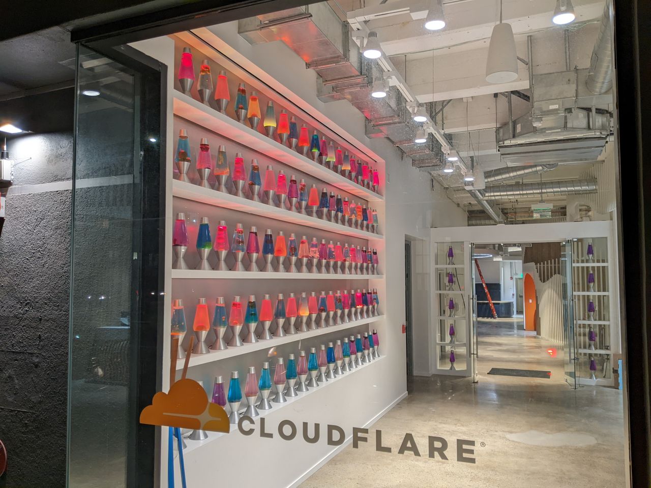
Cloudflare’s wall of lava lamps at 101 Townsend Street, San Francisco. Photo: HaeB, CC BY-SA 4.0

Cloudflare uses a wall of 100 lava lamps as an entropy source
- A camera captures images of the lamps continuously
- The chaotic, unpredictable flow of wax generates random data
- Fed into their secure PRG to seed cryptographic keys
Why lava lamps? They’re a physical process that’s genuinely unpredictable
- Tiny variations in heat, air currents, and wax composition
- No two frames are ever the same
Other companies use different approaches
- Random.org uses atmospheric noise
- Some use radioactive decay or quantum processes

Building a Stream Cipher

How does this help us turn the one-time pad into a more practical cipher?
Let’s encrypt messages up to some maximum length $L$
- How long does the key need to be if we use the original one-time pad?
Let’s pick a short seed value $s$ with length $\ell < L$
Assume that we have a PRG $G$ that maps from $\mathcal{S}$ to $\mathcal{R}$
- $\mathcal{S} = \{0,1\}^\ell$ and $\mathcal{R} = \{0,1\}^L$
What if we replace the key with a pseudo-random number from $G$?
- Key idea: if $G(s)$ is indistinguishable from a truly random key, the cipher should be indistinguishable from the one-time pad!
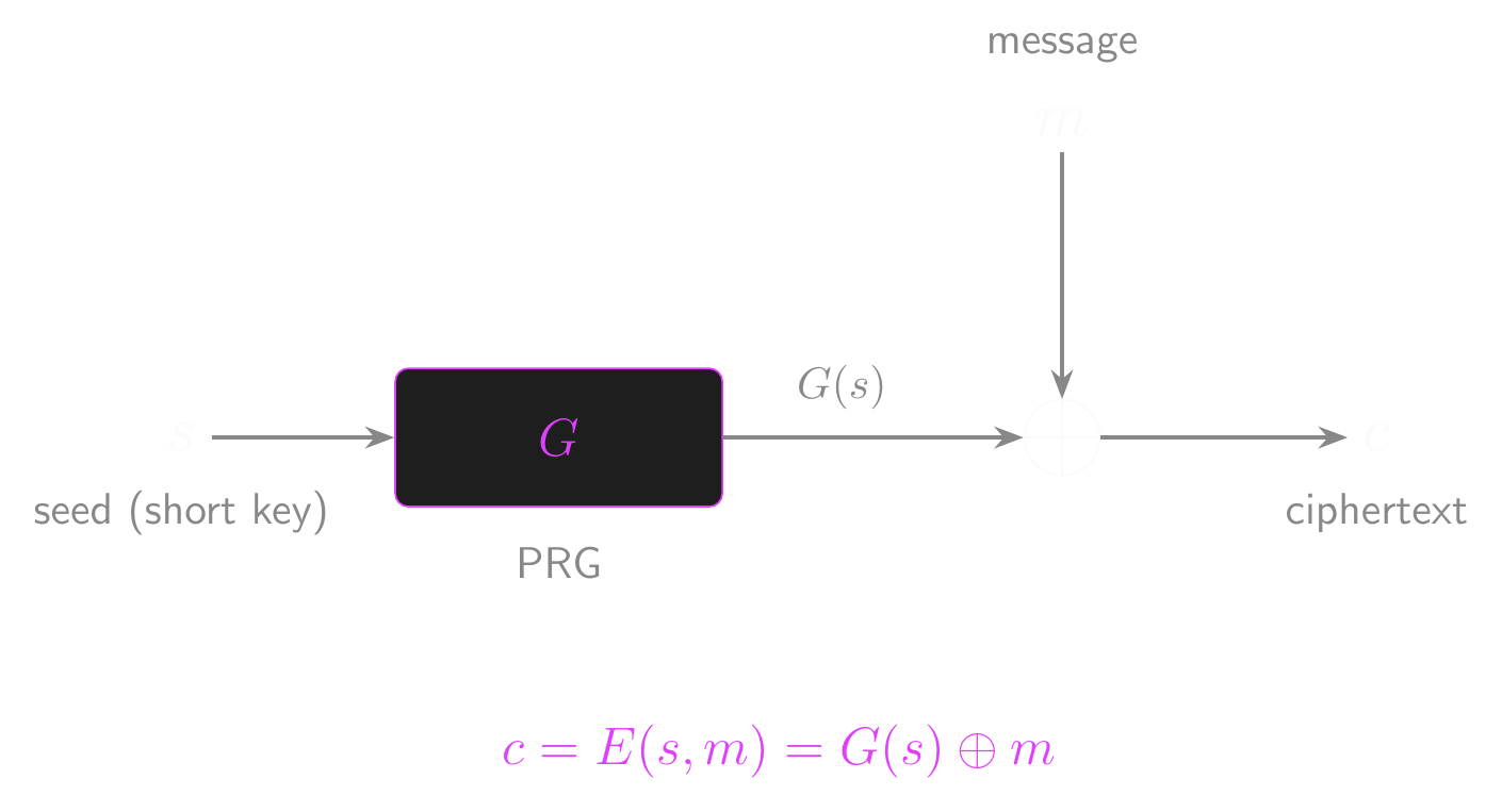
Our stream cipher is defined as:
- $E(s, m) = G(s) \oplus m$
- $D(s, c) = G(s) \oplus c$

Is This Cipher Secure?

Does the correctness property hold? Why (or why not)?
Is it possible for this cipher to be perfectly secure?
- No: $|\mathcal{S}| < |\mathcal{R}|$, so Shannon’s theorem rules it out
Is it possible for this cipher to be semantically secure?

Stream Cipher: Encryption

A Toy Example

Let’s make this concrete with a tiny (insecure!) PRG
Suppose $G : \{0,1\}^4 \to \{0,1\}^8$ and our seed is $s = 1011$
The PRG stretches the seed: $G(s) = G(1011) = 10110011$
We want to encrypt the message $m = 01001110$
Encrypt: $c = G(s) \oplus m = 10110011 \oplus 01001110 = 11111101$
Decrypt: $m = G(s) \oplus c = 10110011 \oplus 11111101 = 01001110$ ✓
The seed is 4 bits but we encrypted an 8-bit message!
- That’s the whole point: short key, long ciphertext
Of course, 4-bit seeds are trivially brute-forced
- We’ll need to talk about how big is big enough

Secure PRGs

Think about this from the attacker’s point of view…
- The security of the cipher hinges on the properties of the PRG
- Can we distinguish between the PRG’s output and true random values?
- Maybe! It depends^TM on the PRG we’re using.
If we can’t tell the difference between $G(s)$ and a truly random $k$…
- With better accuracy than random guessing…
- Then the one-time pad and our stream cipher can’t be distinguished…
- So our stream cipher must be secure!
What’s the catch?
- This is semantic security, not perfect security!
- And it only holds if the PRG is actually secure
- How do we formalise what “secure PRG” means?

PRG Security Intuition

Let’s get some clear ideas about what makes a secure PRG for cryptography
Imagine two scenarios:
- Scenario 0: you receive $G(s)$, where $s$ is a randomly chosen seed
- Scenario 1: you receive $r$, a string chosen uniformly at random from $\mathcal{R}$
A secure PRG is one where no efficient adversary can reliably tell which scenario they’re in
- The two distributions look computationally identical
- If that holds, the PRG is secure!
This might sound pretty familiar…
- Indistinguishable?
- Efficient adversary?
Let’s build a quick guessing game…

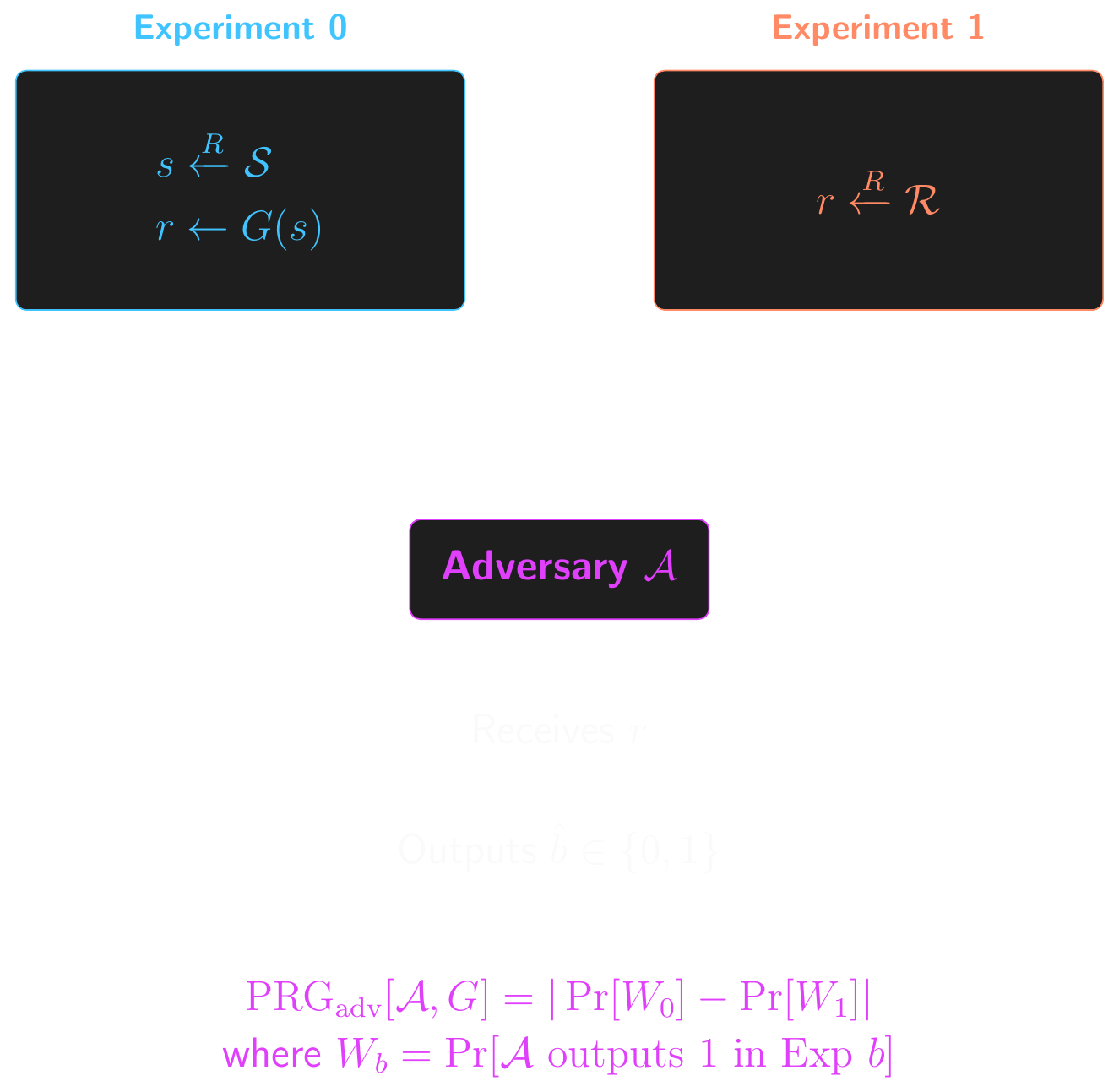
PRG Security: Attack Game

This time around, our attack game will have two sub-games or experiments
- The adversary $\mathcal{A}$ doesn’t know which one they’re playing, and has to guess!
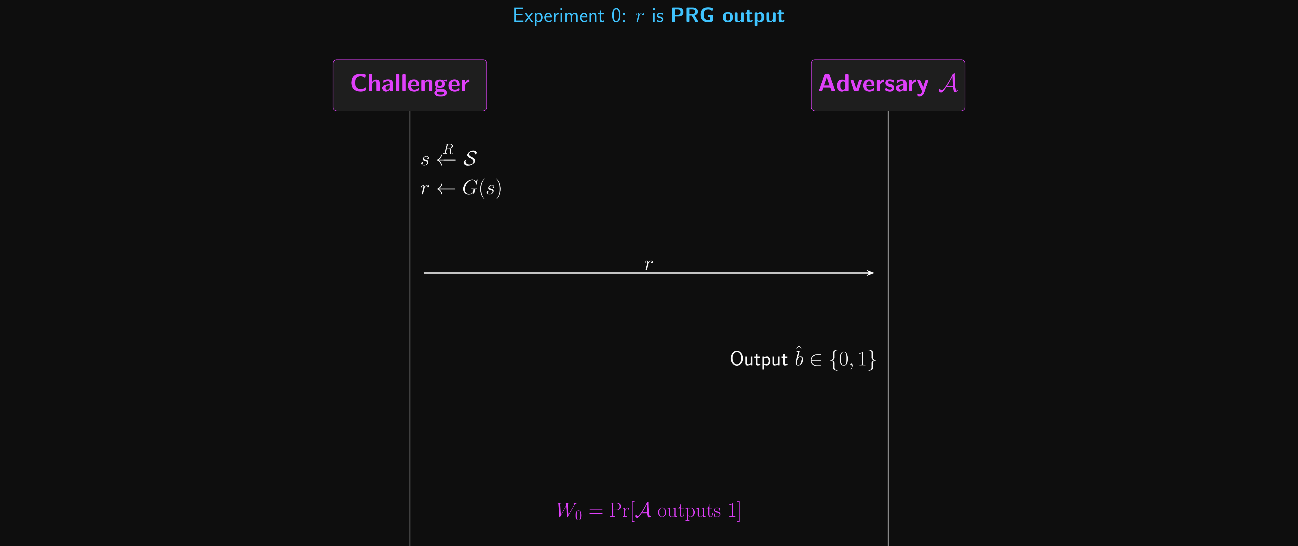
Experiment 0: the challenger computes…
- $s \xleftarrow{R} \mathcal{S}$
- $r \leftarrow G(s)$
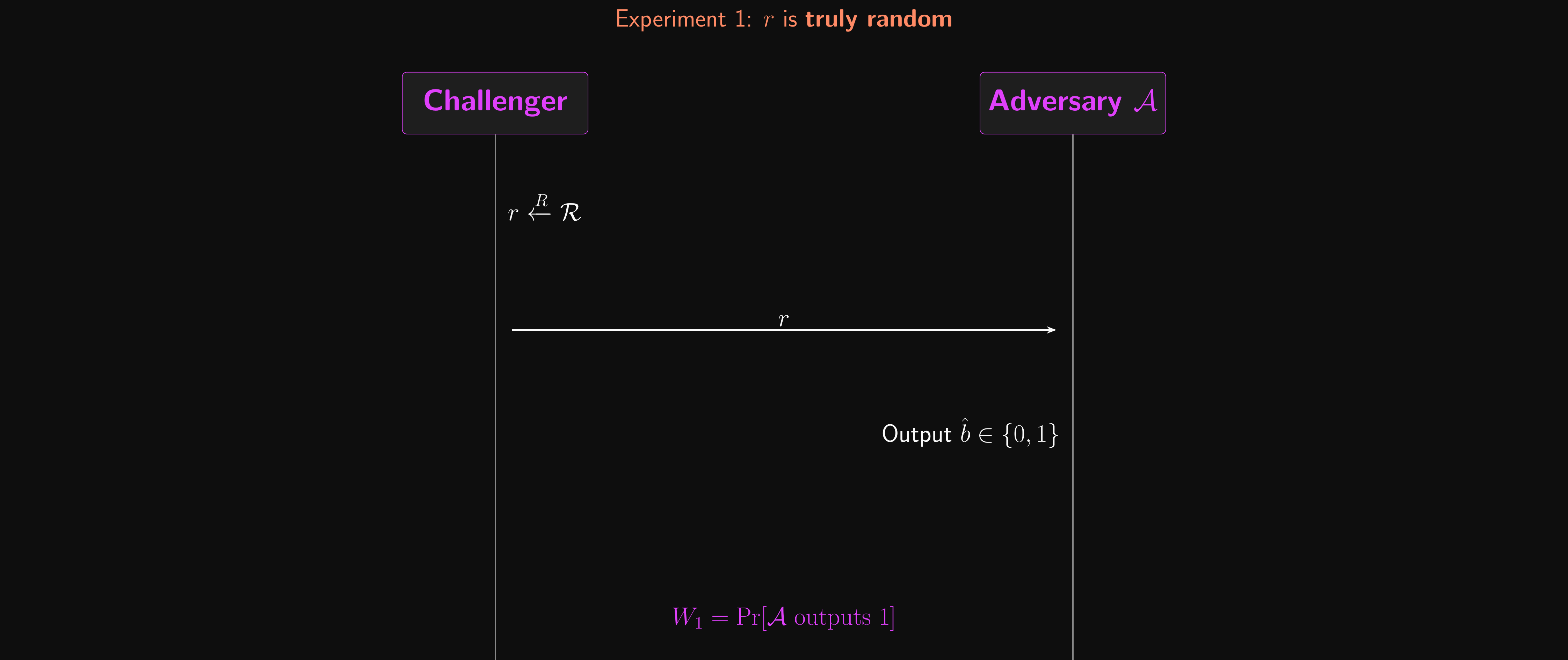
Experiment 1: the challenger computes…
- $r \xleftarrow{R} \mathcal{R}$
$r$ is sent to $\mathcal{A}$, and $\mathcal{A}$ outputs its guess: 0 for “this was PRG output”, 1 for “this was truly random”

Let $W_b$ be the event that $\mathcal{A}$ outputs 1 on Experiment $b$
- $\text{PRG}_\text{adv}[\mathcal{A}, G] = |\Pr[W_0] - \Pr[W_1]|$
- The advantage measures how much better than random guessing (50/50) the adversary can do
- A random guesser has $\Pr[W_0] = \Pr[W_1]$, so the advantage is 0
If $\text{PRG}_\text{adv}[\mathcal{A}, G]$ is negligible for all $\mathcal{A}$, then $G$ is a secure PRG

PRG Security: Attack Game

PRG Security: Experiment 0

PRG Security: Experiment 1

How Big is Big Enough?

There’s one more element needed to make our PRG secure
- Why was it so easy to break the Caesar cipher?
An adversary can always try to brute-force the seed space
- Try every possible seed $s \in \mathcal{S}$, compute $G(s)$, check if it matches
- How long does this take? $|\mathcal{S}|$ operations (one per seed)
If $\ell = 4$: $|\mathcal{S}| = 2^4 = 16$ seeds. Trivial to brute-force.
If $\ell = 40$: $|\mathcal{S}| = 2^{40} \approx 10^{12}$. A fast computer checks this in minutes.
If $\ell = 128$: $|\mathcal{S}| = 2^{128} \approx 10^{38}$. At a billion guesses per second, this takes $10^{29}$ seconds. The universe is only $\approx 4 \times 10^{17}$ seconds old.
The seed length $\ell$ controls how hard it is to break the PRG
- This is a really important idea, so we need to formalise it!

The Security Parameter

The security parameter $\lambda$ is the single number that controls how secure a system is
- In symmetric crypto, $\lambda$ is the key or seed length in bits
- In our stream cipher, the seed length $\ell$ plays the role of $\lambda$
- Everything is parameterised by $\lambda$: key spaces, seed spaces, advantage bounds
We write $\{0,1\}^\lambda$ for the seed/key space, giving $|\mathcal{S}| = 2^\lambda$ possible seeds
Increasing $\lambda$ makes life harder for efficient adversaries
- The work to brute-force grows as $2^\lambda$ (exponential)
- But legitimate operations (encryption, decryption) stay polynomial in $\lambda$
- This gap is what makes computational security possible!
- But a computationally unbounded adversary can always brute-force, no matter how large $\lambda$ is
$\lambda = 128$ is the minimum for symmetric crypto today ($\lambda = 256$ for quantum margin)
When we say an advantage is “negligible”, we mean negligible as a function of $\lambda$

Negligible and Super-Poly

A function $f(\lambda)$ is negligible if it shrinks faster than any inverse polynomial in $\lambda$
- For every positive integer $d$, there exists $\lambda_0$ such that for all $\lambda > \lambda_0$: $f(\lambda) < 1/\lambda^d$
- Intuition: not just small, but vanishingly small. Smaller than $1/\lambda$, $1/\lambda^2$, $1/\lambda^{100}$, …
- Example: $1/2^\lambda$ is negligible. It beats any $1/\lambda^d$ once $\lambda$ is large enough.
The mirror image: $Q(\lambda)$ is super-poly if it grows faster than any polynomial in $\lambda$
- $Q$ is super-poly iff $1/Q$ is negligible
- Otherwise, $Q$ is poly-bounded
- Example: $2^\lambda$ is super-poly. No polynomial $\lambda^d$ can keep up.
Now we can state security precisely:
- “For all efficient adversaries $\mathcal{A}$, $\text{PRG}_\text{adv}[\mathcal{A}, G]$ is negligible in $\lambda$”

Concrete Security

Asymptotic “negligible” guarantees security scales correctly with $\lambda$
- But we deploy at a fixed $\lambda$, so we also need concrete bounds
$b$-bit security: the best known attack needs $\approx 2^b$ operations
- For key search, $T$ trials give advantage $\approx T / 2^b$
Calibrating the scale (advantage shown for a 128-bit key at each attack budget $T$):
- $T = 2^{56}$: cracked on dedicated hardware in hours (DES, 1998); advantage $2^{-72}$
- $T = 2^{64}$: feasible on modern hardware; advantage $2^{-64}$
- $T = 2^{80}$: within reach for well-funded adversaries; advantage $2^{-48}$
- $T = 2^{128}$: advantage $= 1$ (full break), but this is beyond any foreseeable classical computer
128 bits is the minimum acceptable security level for new systems
- This is the concrete reality behind “negligible” at $\lambda = 128$
- Some constructions lose security bits to structural bounds (e.g. birthday attacks)

Seed Space

The seed space is $\mathcal{S} = \{0,1\}^\lambda$, so $|\mathcal{S}| = 2^\lambda$
$2^\lambda$ is super-poly in $\lambda$, so the brute-force probability $1/2^\lambda$ is negligible
A PRG can only be secure if the seed space is super-poly
- Otherwise, an efficient adversary can just enumerate it!
Given a large enough security parameter $\lambda$, our PRG is secure!
All the security definitions we’ve seen work the same way:
- $\text{SS}_\text{adv}$, $\text{PRG}_\text{adv}$, and later $\text{BC}_\text{adv}$, … all must be negligible in $\lambda$

Proving Security

Prove it or it didn’t happen.

Why This Stream Cipher Is Secure

Our stream cipher $\mathcal{E}$ is defined as:
- $E(s, m) = G(s) \oplus m$
- $D(s, c) = G(s) \oplus c$
What’s the only difference between the two?
- Stream cipher uses a PRG to generate the key
- One-time pad uses a truly random key
Secure PRG output is indistinguishable from a random bitstring
- An adversary can only do negligibly better than random guessing
- No useful information about the seed is leaked from the keystream
To have any non-negligible chance at distinguishing ciphertexts…
- …an adversary has to exploit some pattern in the PRG output!

Security Depends on the PRG

The security of a stream cipher is based on $\text{PRG}_\text{adv}[\mathcal{A}, G]$
- If $\text{PRG}_\text{adv}[\mathcal{A}, G]$ is negligible, then $\text{SS}_\text{adv}[\mathcal{B}, \mathcal{E}]$ is negligible
But why is this true? Let’s prove it!

Theorems and Lemmas

Before we dive in, let’s define some terms you’ll see in the textbook
A theorem is a statement that has been proven to be true
- “If the PRG is secure, the stream cipher is semantically secure” is a theorem!
- It has a specific structure: “if [assumptions], then conclusion”
A lemma is a smaller result that helps prove a bigger theorem
- Think of it as a stepping stone: useful on its own, but mainly there to make the main proof easier
- We’ll prove lemmas and then use them as building blocks
A proof shows why a theorem is true, not just that it is
- In cryptography, most proofs are constructive: we build something (an adversary, a simulator) to demonstrate the claim
You won’t need to memorise proofs for the exam
- But understanding the technique behind each proof is important: these patterns recur throughout cryptography

Stream Cipher Security Theorem

Theorem: Let $G$ be a secure PRG. Then the stream cipher $\mathcal{E}$ built from $G$ is semantically secure.
More precisely: for every efficient SS adversary $\mathcal{A}$ attacking $\mathcal{E}$, there exists an efficient PRG adversary $\mathcal{B}$ attacking $G$ such that:
- $\text{SS}_\text{adv}[\mathcal{A}, \mathcal{E}] \leq \text{PRG}_\text{adv}[\mathcal{B}, G]$
In words: anyone who can break the stream cipher can also break the PRG
- PRG is secure (by assumption), so the stream cipher must be too
How do we prove this? We need a new technique…

Proof by Reduction

Our first proof technique: the reduction
The claim: if the PRG $G$ is secure, then the stream cipher $\mathcal{E}$ built from $G$ is semantically secure
How do we prove this? By showing:
- “If you could break the stream cipher, you could use that ability to break the PRG”
- But we assumed the PRG is secure (nobody can break it!)
- So nobody can break the stream cipher either
This is proof by contradiction, with a twist:
- We don’t just say “assume it’s broken”
- We build a specific adversary $\mathcal{B}$ that uses the stream cipher attacker $\mathcal{A}$ as a subroutine
- $\mathcal{B}$ translates $\mathcal{A}$’s ability to break $\mathcal{E}$ into an ability to break $G$

The Reduction

Adversary $\mathcal{B}$ plays the PRG game: receives a challenge string $r$
- $r$ is either $G(s)$ for a random seed $s$, or a truly random string
- $\mathcal{B}$ doesn’t know which!
$\mathcal{B}$ uses $r$ to run an SS game against $\mathcal{A}$:
- $\mathcal{A}$ submits two messages $m_0, m_1$
- $\mathcal{B}$ flips a coin $b \xleftarrow{R} \{0, 1\}$ and computes $c \leftarrow r \oplus m_b$
- $\mathcal{B}$ sends $c$ to $\mathcal{A}$, who outputs a guess $\hat{b}$
- $\mathcal{B}$ outputs 1 (“it was a PRG”) if $\hat{b} = b$, else 0 (“it was random”)

The Reduction: Two Worlds

If $r = G(s)$: $\mathcal{A}$ sees a real stream cipher ciphertext and wins with its usual advantage
If $r$ is truly random: $\mathcal{A}$ sees a one-time pad ciphertext, and its advantage is 0!
- (Recall from L01: the OTP is perfectly secure, so no information about the message is leaked)
$\mathcal{B}$ outputs 1 when $\mathcal{A}$ guesses correctly ($\hat{b} = b$)
- In Exp 0 (PRG): $\mathcal{A}$ is playing a real SS game, so $\Pr[\mathcal{B} \text{ outputs } 1] = \frac{1}{2} + \text{SS}_\text{adv}[\mathcal{A}, \mathcal{E}]$
- In Exp 1 (random): $\mathcal{A}$ is playing against a one-time pad, so $\Pr[\mathcal{B} \text{ outputs } 1] = \frac{1}{2}$
- The gap between these two probabilities is exactly $\text{SS}_\text{adv}[\mathcal{A}, \mathcal{E}]$
Therefore: $\text{PRG}_\text{adv}[\mathcal{B}, G] \geq \text{SS}_\text{adv}[\mathcal{A}, \mathcal{E}]$
- If the left side is negligible (PRG is secure), the right side must be too

The Reduction: Diagram

What Just Happened?

We proved stream cipher security without knowing anything about how $G$ works
- We only used the fact that $G$ is a secure PRG
- This is the power of reductions: they let us build on existing guarantees
The key trick: replacing $G(s)$ with a truly random string turns the stream cipher into a one-time pad
- Real world (PRG output): adversary has some advantage $\epsilon$
- Ideal world (truly random): adversary has advantage 0 (perfect security!)
- The gap between the two worlds is exactly the PRG advantage
This “real world vs ideal world” pattern shows up in nearly every security proof in this course
The real-vs-ideal trick isn’t just for encryption
- We’ll use it for a completely different problem at the end of this lecture

Ghosts of Problems Past

While we’re here, let’s fix the length problem too!
- We can encrypt arbitrary-length messages shorter than the keystream.
- $E(s, m) = G(s)[0 \ldots |m| - 1] \oplus m$
- $D(s, c) = G(s)[0 \ldots |c| - 1] \oplus c$
Have we solved the key length problem?
- Yes!
Have we solved the malleability/integrity problem?
- No!
- But we’ll get back to that one… eventually.
Key reuse was a big problem for the one-time pad
- Does our stream cipher allow for key reuse?
- Try it out and see! Hint: what happens when you XOR two ciphertexts encrypted with the same key?
- We’ll see some possible solutions to this later

The Many-Time Pad (Again)

Remember the many-time pad from L01? The same problem applies here
- Reusing key $s$ means $G(s)$ cancels: $E(s, m_0) \oplus E(s, m_1) = m_0 \oplus m_1$
- An attacker recovers the XOR of the plaintexts, enough for crib-dragging attacks
Our stream cipher inherits this vulnerability directly from the OTP
Real-world examples of this exact mistake:
- Project Venona: the USSR reused one-time pad pages; US/UK intelligence exploited this for decades
- Microsoft PPTP: reused RC4 keystreams, allowing practical plaintext recovery
Key reuse (or nonce reuse) is catastrophic, we’ll need a way to safely encrypt multiple messages with the same key

PRGs all the way down…

Making generators from generators.

Building PRGs from PRGs

Our PRG $G$ maps $\{0,1\}^\lambda \to \{0,1\}^L$, producing $L$ bits of keystream
- But what if our message is longer than $L$ bits?
- Do we need to design a completely new PRG with a bigger output?
We can build larger PRGs from existing ones!
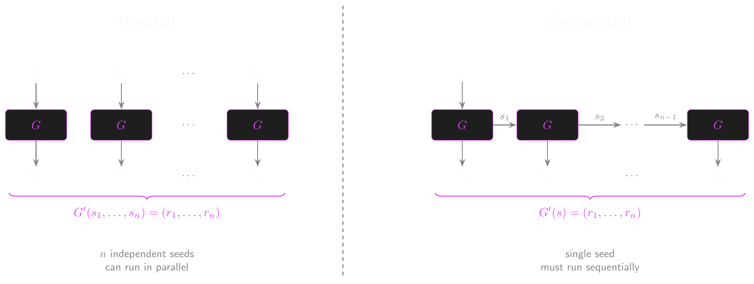
- Two approaches: parallel and sequential composition
- Both produce $n \times L$ bits of output from a PRG that only outputs $L$ bits
- But they have very different tradeoffs
- And we have to be careful not to compromise the security of the PRG!

Parallel Construction

One technique is $n$-wise parallel composition
- We take $n$ independent seeds…
- Generate the output from each seed…
- And concatenate the results into one long output
The new PRG, $G'$, is defined over $(\mathcal{S}^n, \mathcal{R}^n)$
- $G'(s_1, \ldots, s_n) = (G(s_1), \ldots, G(s_n))$ for $(s_1, \ldots, s_n) \in \mathcal{S}^n$
- The repetition parameter, $n$, must be poly-bounded
Is it secure? Can an adversary distinguish it from truly random output?
- Intuitively, an adversary has better odds the more we use the PRG
- $\text{PRG}_\text{adv}[\mathcal{A}, G'] \leq n \cdot \text{PRG}_\text{adv}[\mathcal{B}, G]$
- Security degrades linearly as the repetition parameter increases

Parallel Construction: Seed Size

Note the seed is now $n$ times as long: $(s_1, \ldots, s_n) \in \mathcal{S}^n$
- We need $n \times \lambda$ bits of seed to get $n \times L$ bits of output
- The expansion rate barely improves! Can we do better? (Yes, but first…)
Easy to parallelise: each $G(s_i)$ is independent, so all $n$ can be computed simultaneously
But why does the security bound hold? Let’s prove it!

Proving the Parallel Bound

We claimed $\text{PRG}_\text{adv}[\mathcal{A}, G'] \leq n \cdot \text{PRG}_\text{adv}[\mathcal{B}, G]$. But why?
We can’t directly use a reduction to a single PRG instance (there are $n$ of them!)
Instead, we use a hybrid argument: build a chain of intermediate distributions
- Each adjacent pair in the chain differs in exactly one slot
- If an adversary can tell the endpoints apart, they must be able to tell some adjacent pair apart
- And telling an adjacent pair apart is the same as breaking a single PRG instance!

The Hybrid Chain

Define $n + 1$ hybrid distributions:
- $H_0$: $(G(s_1), G(s_2), \ldots, G(s_n))$ – all real PRG outputs
- $H_1$: $(r_1, G(s_2), \ldots, G(s_n))$ – first slot replaced with random
- $H_2$: $(r_1, r_2, G(s_3), \ldots, G(s_n))$ – first two slots random
- $\quad\vdots$
- $H_n$: $(r_1, r_2, \ldots, r_n)$ – all truly random
The adversary needs to distinguish $H_0$ (all PRG) from $H_n$ (all random)
But $H_0$ and $H_n$ are connected by a chain of $n$ small steps
- Each step changes exactly one slot from PRG output to truly random

Hybrid Chain: A Concrete Example

Let’s try this with $n = 2$ and tiny 4-bit outputs
$H_0 = (G(s_1),\; G(s_2)) = (1011,\; 0110)$ – both from the PRG
$H_1 = (r_1,\; G(s_2))\;\, = (1100,\; 0110)$ – first slot replaced with random
$H_2 = (r_1,\; r_2)\;\;\;\;\;\, = (1100,\; 0011)$ – both truly random
Can you tell $H_0$ from $H_2$?
If not, you shouldn’t be able to spot any single step either
- Each adjacent pair differs in only one slot
- And we’ve already shown that’s a PRG game!

Each Step is a PRG Game

Suppose an adversary can distinguish $H_i$ from $H_{i+1}$
- These differ in only one slot: slot $i + 1$ is $G(s_{i+1})$ in $H_i$ and random $r_{i+1}$ in $H_{i+1}$
We can use this to break $G$ itself:
- Receive challenge $r$ from the PRG game (either $G(s)$ or truly random)
- Fill in slots $1, \ldots, i$ with fresh random values
- Put the challenge $r$ in slot $i + 1$
- Fill in slots $i+2, \ldots, n$ with fresh PRG outputs
- If $r = G(s)$: this looks like $H_i$. If $r$ is random: this looks like $H_{i+1}$.

Completing the Proof

But we assumed $G$ is a secure PRG!
- No efficient adversary can distinguish $G(s)$ from random
- So no efficient adversary can distinguish $H_i$ from $H_{i+1}$ for any $i$
- And if they can’t spot any single step, they can’t spot the overall change from $H_0$ to $H_n$
The total advantage is at most the sum of the $n$ individual advantages
- Each individual step has advantage $\leq \text{PRG}_\text{adv}[\mathcal{B}, G]$
- So the total is $\leq n \cdot \text{PRG}_\text{adv}[\mathcal{B}, G]$
This is why $n$ must be poly-bounded! If $n$ were super-poly, $n \cdot \epsilon$ could stop being negligible

The Hybrid Argument

The hybrid argument is one of the most common proof techniques in cryptography
Recipe for showing two distributions are indistinguishable:
1. Build a chain of hybrids from one distribution to the other
2. Make each adjacent pair differ in exactly one “atomic” step
3. Show that each atomic step reduces to a known hard problem
4. The total advantage is at most the sum of all the individual step advantages
Think of it like a game of “spot the difference”:
- Comparing two photos that differ in 10 places at once is hard
- But if you had 11 photos, each differing from the next in only one place, you could check each pair
- If nobody can spot any single change, nobody can spot the overall difference
We’ll use this technique again when we look at block cipher modes and IND-CPA security

Sequential Construction

The Blum-Micali method (1984, a foundational result in provable pseudorandomness) allows us to chain PRGs sequentially.
This time, take $G$ to be a secure PRG defined over $(\mathcal{S}, \mathcal{R} \times \mathcal{S})$
- Outputs a seed in addition to the usual output!
The new PRG, $G'$, is defined over $(\mathcal{S}, \mathcal{R}^n)$
$G'(s)$:
- $s_0 \leftarrow s$
- $\textbf{for } i = 1 \textbf{ to } n \textbf{ do: } (r_i, s_i) \leftarrow G(s_{i-1})$
- $\textbf{return } (r_1, \ldots, r_n)$

Sequential Construction: Properties

$G'$ is the $n$-wise sequential composition of $G$
The big win: only ONE seed of $\lambda$ bits, but $n \times L$ bits of output!
- Much better expansion rate than parallel composition
- This is essentially how real stream ciphers work
Downside: inherently sequential (each step needs the previous seed)
- But ChaCha20 cleverly avoids this by using a counter instead of chaining seeds
- The counter gives both sequential structure (for security) and random access (for parallelism)
The security bound is similar to the parallel case (also provable by hybrid argument)
- $\text{PRG}_\text{adv}[\mathcal{A}, G'] \leq n \cdot \text{PRG}_\text{adv}[\mathcal{B}, G]$

PRG Composition: Parallel vs Sequential

Expansion Rate

We can evaluate PRGs by their expansion rate
How much does it “stretch” the seed into the output?
A PRG with a $\lambda$-bit seed and $L$-bit output has an expansion rate of $L / \lambda$
Or we can use the seed space and output space to express it as
- $\log |\mathcal{R}| / \log |\mathcal{S}|$
Parallel composition: $n \times L$ bits of output from $n \times \lambda$ bits of seed
- Expansion rate: $(n \times L) / (n \times \lambda) = L / \lambda$, no improvement!
Sequential composition: $n \times L$ bits of output from just $\lambda$ bits of seed
- Expansion rate: $(n \times L) / \lambda$, scales linearly with $n$!

Real-World Stream Ciphers

From state-of-the-art to cautionary tale.

Let’s Build!

Usually, this would be the part where we implement some kind of toy stream cipher
- Great for a hands-on example, but riddled with flaws
But I’ve been impressed so far… so let’s build a state-of-the-art stream cipher!
And when I say stream cipher…
- I mean a pseudo-random generator
- With an XOR operation tacked on at the end
Obligatory reminder: DON’T ROLL YOUR OWN CRYPTO
- We’re implementing a cipher to learn by doing!
- The cipher is secure
- Your implementation isn’t necessarily secure!

Cryptographic Nonce

Remember: the basic stream cipher $E(s, m) = G(s) \oplus m$ is deterministic
- Encrypting the same message twice produces the same ciphertext!
- It’s only safe for a single message per key
A nonce (“number used only once”) breaks that determinism
- Generally doesn’t have to be secret (unlike a key)
- Generally doesn’t have to be unpredictable (unlike an IV)
- But it does have to be unique!
We’ll encounter IVs (initialization vectors) next week!
- Some sources will also call IVs nonces, so caveat lector.

Nonces and Multi-Message Security

Adding a nonce extends a PRG into a primitive that produces a unique keystream for each (key, nonce) pair
- We’ll formally define this as a pseudorandom function (PRF) next week
- For now: think of it as a PRG that takes both a key and a counter as input
This allows multiple messages to be safely encrypted with the same key!
- Only if each key-nonce pair is used only once
- Nonce reuse breaks security! (Same key + same nonce = same keystream)
Each key-nonce pair produces a unique keystream
- This is the difference between single-message and multi-message security
- We’ll formalise this as IND-CPA security next week with block cipher modes

Salsa and ChaCha

We’re going to take a different approach to the parallel and sequential compositions we looked at earlier.
Instead, we’re going to build a pseudorandom function in counter mode.
Salsa and ChaCha are related families of fast stream ciphers.
- Used as part of protocols like TLS and SSH
- Specifically, we’re going to implement ChaCha20
ChaCha20 takes a 256-bit key as input
- Represented as 8 32-bit words (a word is a fixed-size data unit, typically 32 bits)
It also takes a second input: a 64-bit nonce
- Represented as 2 32-bit words

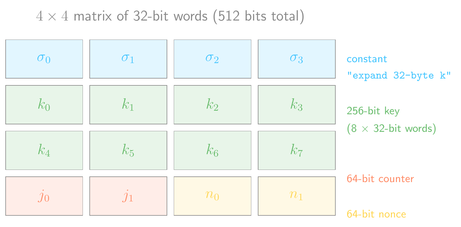
State Initialization

The initial state for ChaCha20 is a $4 \times 4$ matrix of 32-bit words constructed from:
- $\sigma$ = "expand 32-byte k" (128-bit constant, four 32-bit words)
- $k$ (256-bit key, eight 32-bit words)
- $j$ (64-bit counter, two 32-bit words)
- $n$ (64-bit nonce, two 32-bit words)
Remember, this doesn’t have to be implemented as a 2-dimensional array!

ChaCha20: State Matrix

Permutation

The permutation $\pi : \{0, 1\}^{512} \to \{0, 1\}^{512}$ is made up of a fixed number of rounds
- ChaCha20 runs 20 rounds in total (hence the name)
A quarter-round function is applied four times per round, covering all 16 state words
- Odd rounds execute column-wise over the working state matrix
- Even rounds execute diagonal-wise over the working state matrix
The full spec can be found in RFC 7539
- RFC 7539 — ChaCha20 and Poly1305
- Note that the RFC uses a 32-bit counter and 96-bit nonce
Finally, the initial state matrix is added to the working state matrix (word-wise, $\bmod 2^{32}$)
- Without this step, the permutation could be inverted to recover the key!
- The result is a 512-bit pseudo-random output block
Counter value $j$ produces keystream block $j$, enabling direct random access to any block
- Random access and parallel computation are possible!

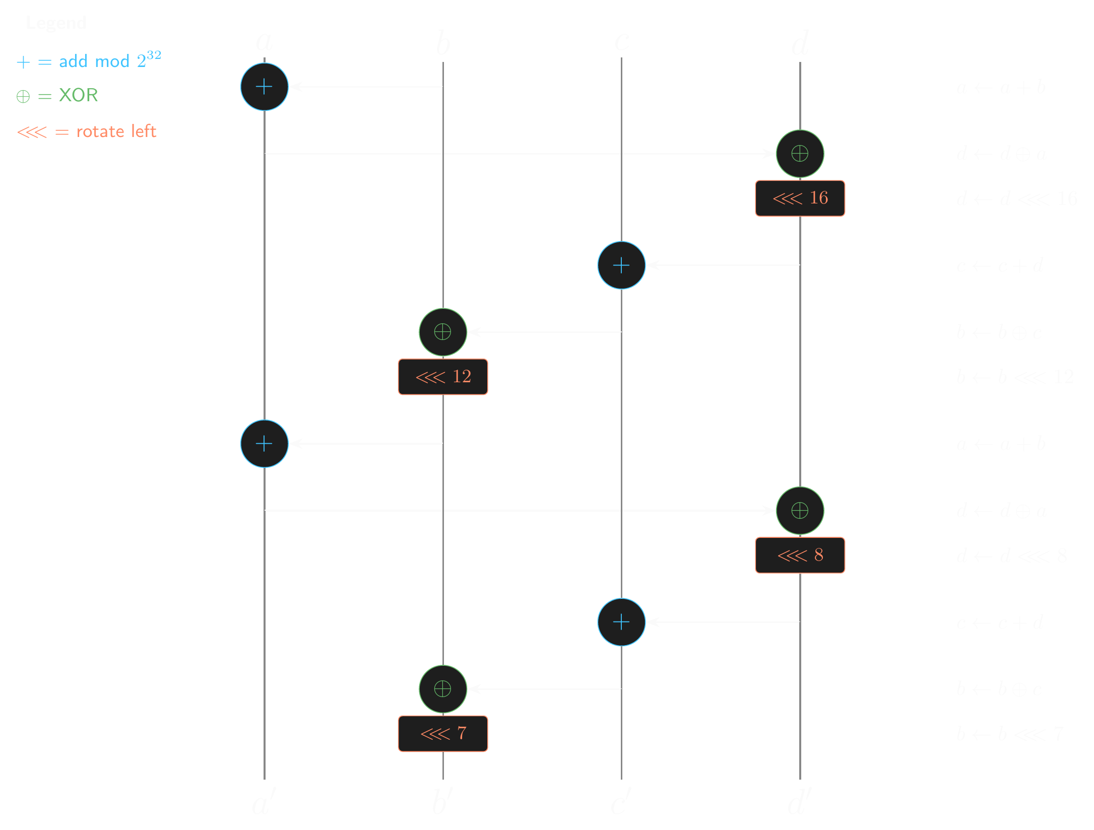
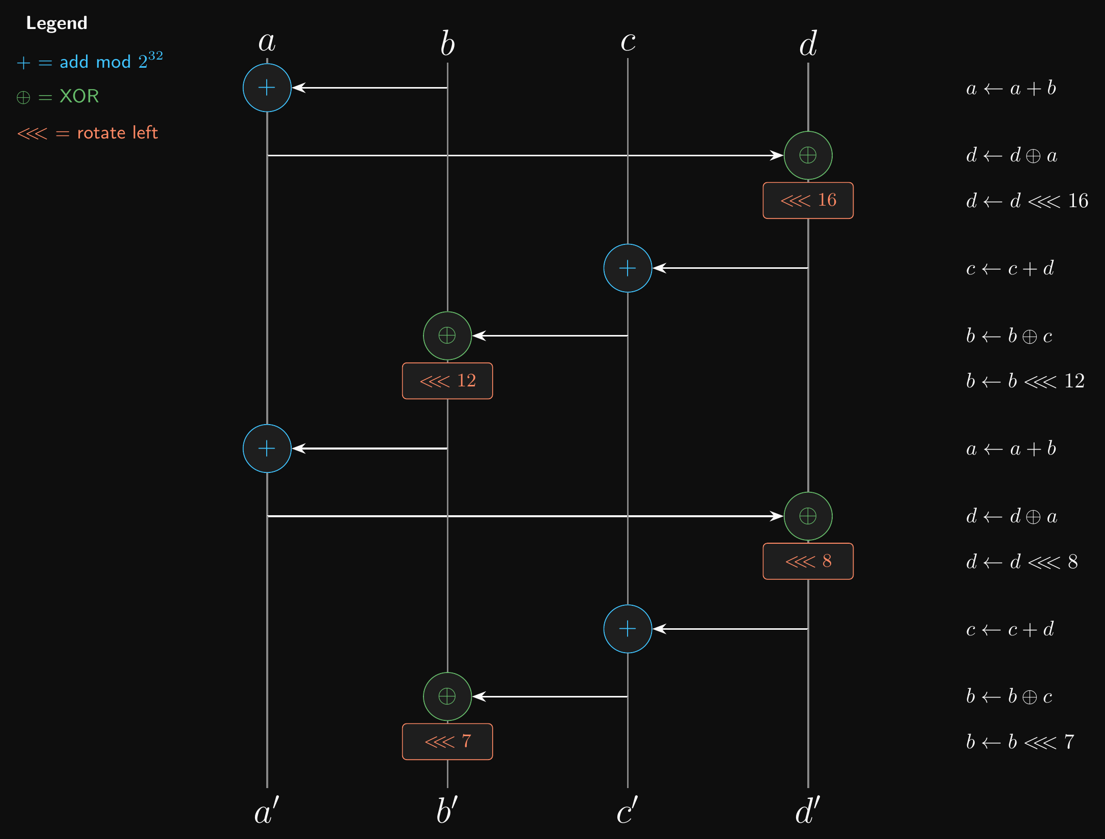
Quarter Round Function

The quarter round function is made up of addition, XOR and rotation operations
Easy to implement in software or hardware
It’s an ARX algorithm (Add-Rotate-XOR)
- Each ARX step has the form: $a \mathrel{+}= b$; then $d \mathrel{\oplus}= a$; then $d \text{ <<<}= n$
- The quarter-round chains four such steps together, mixing all four input words
- $+$ is modular addition $\bmod 2^{32}$, $\text{<<<}$ is rotate left
Constant-time operations, no branching
- Resistant to timing attacks

ChaCha20: Quarter-Round Function

RC4

Sometimes called ARCFOUR or ARC4 - “alleged” RC4
- Leaked from, but never acknowledged by, RSA Security
- The author (Ron Rivest) eventually confirmed it in a 2014 paper
- Yes, that RSA Security! They’ll pop up a few more times in other lectures.
Popular at the time!
- Simple to implement, easy to apply
- No need to worry about modes of operation, block sizes or padding
- Very fast: comparable to AES, much faster than 3DES
Some built-in OS secure PRGs (CSPRNGs) used RC4
Let’s look at how it actually works

RC4: Key Scheduling Algorithm (KSA)

RC4’s internal state is a permutation of the integers $0, 1, \ldots, 255$
- 256 bytes of state, often called the “S-box”
The KSA initialises this permutation using the key $k$:
- $\textbf{for } i = 0 \textbf{ to } 255 \textbf{ do: } S[i] \leftarrow i$
- $j \leftarrow 0$
- $\textbf{for } i = 0 \textbf{ to } 255 \textbf{ do:}$
  - $j \leftarrow (j + S[i] + k[i \bmod |k|]) \bmod 256$
  - $\text{swap}(S[i], S[j])$
Only 256 swaps, regardless of key length
Short keys (e.g. 40-bit WEP keys) repeat cyclically
- Many elements barely move from their initial position

RC4: Keystream Generation (PRGA)

Once the state is initialised, keystream bytes are generated one at a time:
- $i \leftarrow 0, \; j \leftarrow 0$
- $\textbf{for each output byte:}$
  - $i \leftarrow (i + 1) \bmod 256$
  - $j \leftarrow (j + S[i]) \bmod 256$
  - $\text{swap}(S[i], S[j])$
  - $\textbf{return } S[(S[i] + S[j]) \bmod 256]$
Each output byte depends on the current state of the permutation
The state evolves incrementally: each byte depends on all previous state
- No random access, no parallelism (contrast with ChaCha20!)
Beautifully simple: fits in a few lines of code

Why RC4 is Broken

Biased early outputs: The KSA doesn’t mix the state enough
- The second output byte equals 0 with probability $\approx 1/128$ instead of $1/256$
- This bias in the first bytes leaks information about the key
- Even dropping the first 256 bytes doesn’t fully fix the problem
No nonce input: Same key always produces the same initial state and keystream
- WEP concatenated the key with a 24-bit IV: only $2^{24} \approx 16$ million possible keystreams per key
- This is exactly the many-time pad problem!
Statistical biases throughout: Long-range correlations in the keystream
- Practical plaintext recovery demonstrated against TLS (2013, 2015)
Prohibited from use with TLS since 2015
- Ironically, it was previously recommended as a workaround for the BEAST attack (a 2011 CBC-mode attack on TLS… we’ll cover CBC next week)
Don’t use RC4!

Randomness

A user’s guide.

Classes of RNGs

The secure PRGs we’ve discussed so far are also called CSPRNGs
- Cryptographically Secure Pseudo-Random Number Generators
- Be careful not to get these mixed up! Not all PRGs are secure
- Picking the wrong kind of RNG for a task can have dire consequences
True RNGs (TRNGs) are actually random, but expensive!
- Usually used to seed a cheaper CSPRNG

Attacking RNGs

A CSPRNG needs to do everything a normal PRNG can do
That means passing rigorous statistical tests!
E.g. the next-bit test: an attacker shouldn’t be able to guess the next generated bit
- …even if they know every bit that came before it!
In polynomial time, the best they can do is negligibly better than a 50-50 guess
- Sound familiar?
If you know the state of a PRNG, then you can figure out the next output
- You might also be able to figure out past outputs (and the seed)
A good CSPRNG must not reveal past outputs…
- …even if its state is fully or partially compromised!
Some routers seeded their RNG from the time since boot, giving an attacker a tiny, predictable seed space, brute-forceable in seconds

What CSPRNG should we use?

Most/all of you will probably use one in your projects!
Probably some built-in secure random number generator (I hope…)
- Python and Web Crypto both provide these
Under the hood, most of these hook into the OS’s RNG
- E.g. /dev/random and /dev/urandom on Linux
- These use real sources of entropy with a CSPRNG based on ChaCha20
Please don’t roll your own CSPRNG!
Rolling your own PRNG for a game or other non-security context should be fine
- But maybe not for research purposes or Monte Carlo simulations…
If you want to try your hand at creating a PRNG, test it!
- Use a well-known battery of statistical tests like TestU01
- But remember, passing statistical tests doesn’t imply security!
- It’s sine qua non (necessary but not sufficient): passing statistical tests is required, but it doesn’t imply security

When RNG goes bad

Can you really trust your standard library?

Bad PRNGs

java.util.Random has always used a linear congruential generator (LCG), and still does
- Java 17 introduced RandomGenerator with better algorithms, but you have to opt in
LCGs were already known to be poor, but the default stayed anyway
LCGs are fast and don’t need much memory
Completely unsuitable for cryptography (of course)
Problems get really obvious with multi-dimensional data

Linear Congruential Generators

Let’s build a PRNG!
LCGs are old and well-known. They’re also easy to implement!
All you need to do is implement this recurrence relation:
- $X_{n+1} = (a \cdot X_n + c) \mod m$, where $X_0$ is the seed value
The seed, multiplier and increment must be less than the modulus!
There are a bunch of different subtypes
Let’s implement RANDU
- Set $a = 65539$, $c = 0$, $m = 2^{31}$
LCGs are sensitive to parameter choice
- The LCG will repeat after a parameter-dependent period
- The quality of the RNG will vary wildly depending on the parameters!
RANDU used to be widely used, but it’s laughably poor
- May have wrecked lots of scientific papers

And this is why it’s bad!

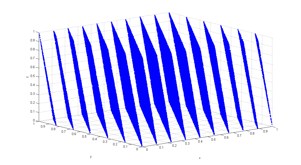
100,000 consecutive triples from RANDU plotted in 3D. The points fall on just 15 parallel planes. Image: Luis Sanchez, CC BY-SA 3.0

RANDU: 15 Parallel Planes

RANDU satisfies: $X_{n+2} = 6 X_{n+1} - 9 X_n \pmod{2^{31}}$
- Every output is a linear combination of the previous two
- That’s why the points fall on 15 parallel planes!
A truly random source would fill the cube uniformly
- RANDU’s output has massive, visible structure
This is exactly the kind of pattern a statistical test (or an attacker) can detect
- And why choosing good parameters for even a simple PRNG matters!

Mersenne Twister

Mersenne Twister is a decent general-purpose PRNG
Huge period of $2^{19937} - 1$ (a Mersenne prime, hence the name)
- A Mersenne prime is a prime of the form $2^p - 1$ (which requires $p$ itself to be prime, but that alone isn’t enough: $2^{11} - 1 = 2047 = 23 \times 89$)
Relatively high memory requirements
Passes most (but not all) standard test suites for statistical randomness
Used as the default in many programming languages and libraries
- Even in some versions of Microsoft Excel
Not cryptographically secure!
- After observing just 624 consecutive outputs, an attacker can fully reconstruct the internal state
- All future (and past) outputs become predictable

Xorshift

Xorshift is a family of PRNGs
Fast, very simple to implement, low memory requirements
With some modifications, can pass most statistical tests
- But only once a non-linear step is added!
Fits in a single screen’s worth of C code

Quis custodiet ipsos custodes?

We can’t talk about RNG in cryptography without mentioning that there have been several standards published and later withdrawn
- Some that didn’t work as intended
- And some that did work as intended, just not as expected…
Most notoriously, Dual_EC_DRBG, published by NIST
- DRBG? Deterministic Random Bit Generator, i.e. a PRNG
- EC? Because it’s built using elliptic curves.
- Usually associated with asymmetric cryptography.
- Unusual for a PRNG…
No security proof was published
- Just a suggestion that it would be hard to crack
You can probably guess what’s coming next!

The Dual_EC_DRBG Backdoor

Turns out that the standard was mostly written by the NSA
And the NSA secretly paid RSA Security $10m to include it as a default in their cryptographic library
Why? Because Dual_EC_DRBG has a possible backdoor…
- The generator uses two elliptic curve points $P$ and $Q$ whose relationship was chosen by the NSA
- If you know the discrete log $e$ such that $Q = eP$, you can recover the internal state from a short output
- Only the NSA knew $e$, so only the NSA could decrypt traffic using the backdoored generator
Major embarrassment for NIST (and everyone else involved)
- The standard has been withdrawn since
OpenSSL’s implementation, amusingly, never actually worked

Commit to the Bit

PRGs aren’t just for encryption.

Heads or Tails?

Ever flipped a coin with someone?
Easy for both parties to have mutual trust!
- One person calls heads or tails
- The other person flips the coin
Both of them can hear the call and verify the result of the toss
- No way for anyone to cheat it
- Even with an unfair coin, you don’t know if the call will be heads or tails
This isn’t so easy if you’re not in the same place…
If Alice tosses the coin knowing what Bob’s guess is…
- She can cheat!
But if Bob only reveals his guess after he knows the result of the toss…
- He can cheat!
And neither of them can trust the result…

Bit Commitment

Let’s try to fix the coin toss protocol with some very practical™ cryptography!
Bob needs to be able to commit to a guess - heads or tails, 0 or 1
- Bob needs to be able to send a commitment string to Alice
- It shouldn’t give Alice any information about Bob’s guess
  - This is the hiding property
Even if Alice rigs the coin toss, she doesn’t have a better chance of winning
- Getting heads 100% of the time isn’t useful
- Bob has a 50% chance of guessing heads, so the odds are the same!
Bob needs to be able to prove what his guess was after the toss
- Bob sends Alice an opening string
- Alice uses it to extract the guess from the commitment string
- Bob shouldn’t be able to change his guess!
  - This is the binding property

PRGs to the Rescue

That’s all well and good, but how can we actually implement it?
Bob commits to a bit $b_0 \in \{0, 1\}$
Alice picks a random $r \in \mathcal{R}$ and sends $r$ to Bob first
- Why first? If Bob chose $r$, he could cheat (we’ll see why in the binding proof)
Bob picks a random $s \in \mathcal{S}$ and computes $c \leftarrow \text{com}(s, r, b_0)$
- $\text{com}(s, r, b_0) = G(s)$ if $b_0 = 0$
- $\text{com}(s, r, b_0) = G(s) \oplus r$ if $b_0 = 1$
Bob sends the commitment string $c$ to Alice

Opening the Commitment

After the toss, Bob sends his guess $b_0$ and the opening string $s$ to Alice
Alice verifies that $c = \text{com}(s, r, b_0)$
- If they match, she accepts that Bob’s guess was $b_0$
- Otherwise, she rejects it

Hiding Property

The hiding property follows directly from PRG security!
- $G(s)$ is computationally indistinguishable from a random $r \in \mathcal{R}$
- And therefore $G(s) \oplus r$ is too
- So Alice can’t know what Bob’s guess is
That was easy!

Binding Property: Setup

The binding property is a bit harder to show, and needs some constraints!
- We require that $1 / |\mathcal{S}|$ be negligible, i.e. that $|\mathcal{S}|$ be super-poly
- And we require that $|\mathcal{R}| \geq |\mathcal{S}|^3$ (we’ll see why in a moment)
If Bob wants to cheat, he needs an opening string that can open to be 0 or 1
- He needs to find $s_0, s_1 \in \mathcal{S}$ s.t. $c = G(s_0) = G(s_1) \oplus r$
- $\Rightarrow G(s_0) \oplus G(s_1) = r$
A “bad $r$” is one where some $s_0, s_1 \in \mathcal{S}$ exist to satisfy that equation.
How many possible pairs of seeds can produce a bad $r$?

Binding Property: Counting Argument

There are $|\mathcal{S}| \cdot |\mathcal{S}| = |\mathcal{S}|^2$ possible pairs of seeds
- Each pair $(s_0, s_1)$ determines exactly one potential bad $r$: the value $G(s_0) \oplus G(s_1)$
- So there are, at worst, $|\mathcal{S}|^2$ distinct bad $r$ values
How likely is it that Alice picks a bad $r$ at random?
$\frac{|\mathcal{S}|^2}{|\mathcal{R}|} < \frac{|\mathcal{S}|^2}{|\mathcal{S}|^3} = \frac{1}{|\mathcal{S}|}$
$1 / |\mathcal{S}|$ is negligible (by our constraint), so the binding property holds!
The probability that Bob can cheat vanishes as the seed space grows

Bit Commitment

This scheme isn’t perfect…
- You can attack it at the protocol level
- But it’s a pretty simple scheme and a neat use of PRGs
- There are better bit commitment schemes out there if you ever need one!
Lots of cryptographic primitives can be used in unexpected ways
- In more complex schemes to achieve different goals
- Or to build other cryptographic primitives
- We’ll see more of these in future lectures!

Conclusion

What did we learn?

So, what did we learn?

Stream ciphers use a PRG to stretch a short key into a long keystream
- $E(s, m) = G(s) \oplus m$
The security parameter $\lambda$ controls the level of security
- Advantages must be negligible in $\lambda$; seed/key spaces must be super-poly
A PRG is secure if its output is computationally indistinguishable from random
- Formalised via the PRG security game (Experiment 0 vs Experiment 1)
Proof by reduction: if the PRG is secure, the stream cipher is semantically secure
PRGs can be composed in parallel or sequentially to produce longer outputs
- The hybrid argument proves that security degrades linearly with $n$

So, what did we learn? (cont.)

ChaCha20 is a modern, widely-used stream cipher (TLS, SSH)
- Uses a nonce to safely encrypt multiple messages with the same key
Not all PRNGs are created equal!
- CSPRNGs for cryptography, regular PRNGs for everything else
- Bad parameter choices and backdoors have caused real-world failures
Stream ciphers protect against passive eavesdroppers, but not against active attackers who can modify ciphertexts. We’ll close that gap later with authenticated encryption.
PRGs can also be used for non-encryption tasks like bit commitment

For next time…

Complete the challenges in this week’s tutorial!
- No grade this time, just bragging rights.
- And stuff from the tutorials might be helpful later on…
We’ll take a look at block ciphers next week.
Complete some assigned reading for next week:
- Chapter 7 of Crypto 101
- Sections 3.1 to 3.3 of Applied Cryptography
- And 3.9 if you’re interested in RC4
- The rest of the chapter is interesting, but only if you’ve got time
- I don’t expect you to learn off proofs from the textbook!

Questions?

Ask now, catch me after class, or email eoin@eoin.ai